Stack

Build via Axes

A histogram stack holds multiple 1-D histograms into a stack, whose axes are required to match. The most common way to create one is with a categorical axes:

import matplotlib.pyplot as plt
import numpy as np

import hist
from hist import Hist

ax = hist.axis.Regular(25, -5, 5, flow=False, name="x")
cax = hist.axis.StrCategory(["signal", "upper", "lower"], name="c")
full_hist = Hist(ax, cax)

full_hist.fill(x=np.random.normal(size=600), c="signal")
full_hist.fill(x=2 * np.random.normal(size=500) + 2, c="upper")
full_hist.fill(x=2 * np.random.normal(size=500) - 2, c="lower")


s = full_hist.stack("c")

You can build this directly with hist.Stack(h1, h2, h3), hist.Stack.from_iter([h1, h2, h3]), or hist.Stack.from_dict({"signal": h1, "lower": h2, "upper": h3}) as well.

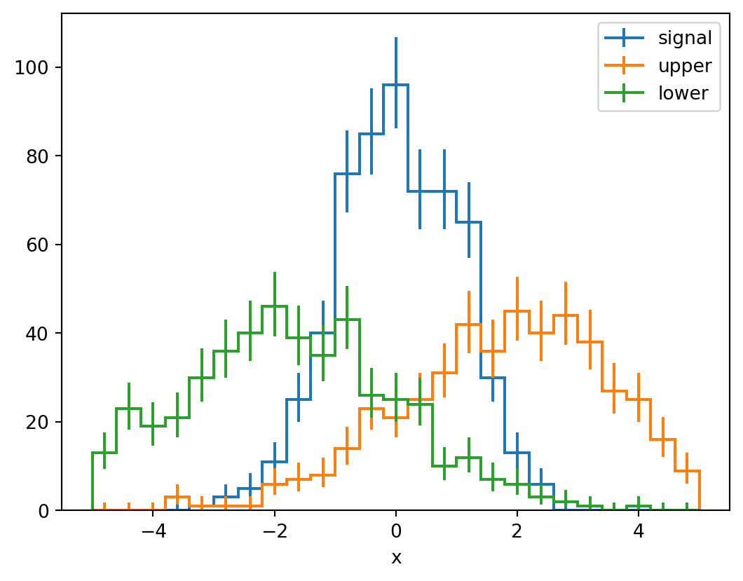
HistStack has .plot() method which calls mplhep and plots the histograms in the stack:

s.plot()
plt.legend()
plt.show()

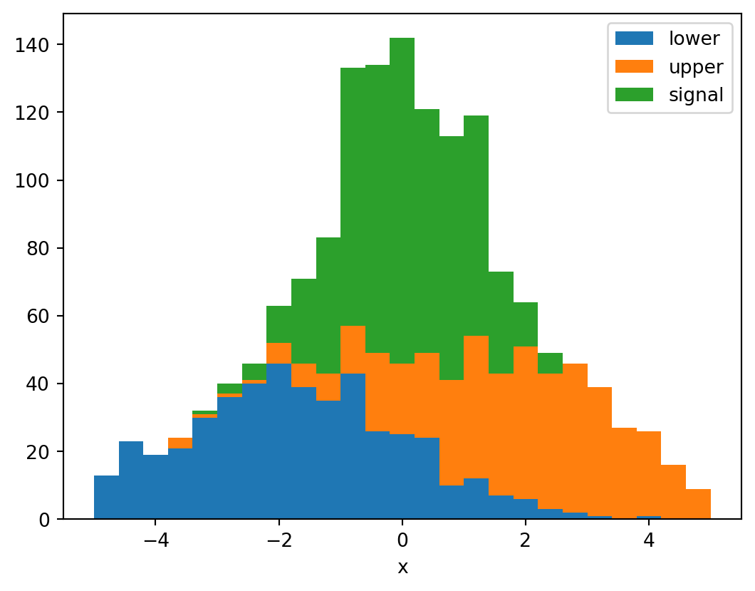
For the “stacked” style of plot, you can pass arguments through to mplhep. For some reason, this reverses the graphical order, but we can easily undo that by applying a slicing operation to the stack:

s[::-1].plot(stack=True, histtype="fill")
plt.legend()
plt.show()

We can use .show() to access histoprint and print the stacked histograms to the console.

Note: Histoprint currently supports only non-discrete axes. Hence, it supports only regular and variable axes at the moment.

s.show(columns=120)

 -5.000 _                                                                                                      157/row ╷
 -4.600 _═════════
 -4.200 _══════════════
 -3.800 _═════════════════════
 -3.400 _═════════════════════
 -3.000 _══════════════════════
 -2.600 _██══════════════════════════
 -2.200 _███││││═════════════════════════════
 -1.800 _███████││══════════════════════════════
 -1.400 _█████████████████████│││││││═══════════════════════════════
 -1.000 _██████████████████████████████████│││││││││═════════════════════
 -0.600 _██████████████████████████████████████████████████│││││││││││═══════════════════════
 -0.200 _██████████████████████████████████████████████████████████████│││││││││││││═══════════════════
  0.200 _█████████████████████████████████████████████████████████████████│││││││││││││││══════════════════
  0.600 _███████████████████████████████████████████████████████████████████████││││││││││││││││││││││││││═════════════
  1.000 _██████████████████████████████████████████████│││││││││││││││═══════
  1.400 _████████████████████████│││││││││││││││││││││││═══════
  1.800 _█████████████████││││││││││││││││││││││││││═══
  2.200 _███████████│││││││││││││││││││││││││││││════
  2.600 _███│││││││││││││││││││││││││═
  3.000 _█││││││││││││││││││││││││││══
  3.400 _█││││││││││││││││││││││││││││││││═══
  3.800 _││││││││││││││││││││││
  4.200 _││││││││││││
  4.600 _││││││││││
  5.000 _││││││││││││
                                             █ signal    │ upper     ═ lower

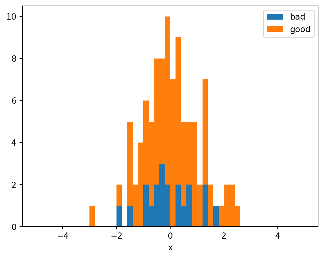
Manipulations on a Stack

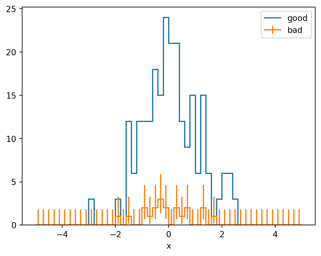
h = Hist.new.Reg(50, -5, 5, name="x").StrCat(["good", "bad"], name="quality").Double()

h.fill(x=np.random.randn(100), quality=["good", "good", "good", "good", "bad"] * 20)

# Turn an existing axis into a stack
s = h.stack("quality")
s[::-1].plot(stack=True, histtype="fill")
plt.legend()
plt.show()

Histograms in a stack can have names. The names of histograms are the categories, which are corresponding profiled histograms:

print(s[0].name)
s[0]

good

Regular(50, -5, 5, name='x')

---

Double() Σ=80.0

You can use those names in indexing, just like for axes (only when using string names):

print(s["bad"].name)
s["bad"]

bad

Regular(50, -5, 5, name='x')

---

Double() Σ=20.0

You can scale a stack:

(s * 5).plot()
plt.legend()
plt.show()

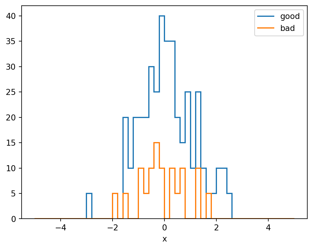
Or an item in the stack inplace:

s["good"] *= 3
s.plot()
plt.legend()
plt.show()

You can project on a stack, as well, if the histograms are at least two dimensional. h.stack("x").project("y") is identical to h.project("y").stack("x").