Interpolation#
Via SciPy#
We can perform interpolation in Hist using SciPy.
[1]:
# Make the necessary imports.
import matplotlib.pyplot as plt
import numpy as np
from scipy import interpolate

from hist import Hist
[2]:
# We obtain evenly spaced numbers over the specified interval.
x = np.linspace(-27, 27, num=250, endpoint=True)

# Define a Hist object and fill it.
h = Hist.new.Reg(10, -30, 30).Double()
centers = h.axes[0].centers
weights = np.cos(-(centers**2) / 9.0) ** 2
h.fill(centers, weight=weights)
[2]:
Regular(10, -30, 30, label='Axis 0')
Double() Σ=5.596329884235402
Double() Σ=5.596329884235402
Linear 1-D#
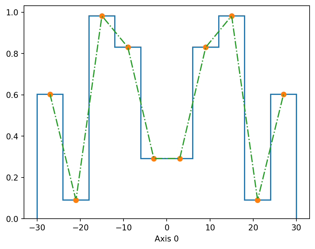
We can obtain a linear interpolation by passion the kind="linear" argument in interpolate.interp1d().
[3]:
linear_interp = interpolate.interp1d(h.axes[0].centers, h.values(), kind="linear")
[4]:
h.plot()  # Plot the histogram
plt.plot(h.axes[0].centers, h.values(), "o")  # Mark the bin centers
plt.plot(x, linear_interp(x), "-.")  # Plot the Linear interpolation
plt.show()
Cubic 1-D#
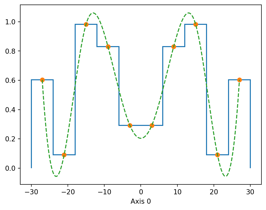
We can obtain a cubic interpolation by passion the kind="cubic" argument in interpolate.interp1d().
[5]:
cubic_interp = interpolate.interp1d(h.axes[0].centers, h.values(), kind="cubic")
[6]:
h.plot()  # Plot the histogram
plt.plot(h.axes[0].centers, h.values(), "o")  # Mark the bin centers
plt.plot(x, cubic_interp(x), "--")  # Plot the Cubic interpolation
plt.show()
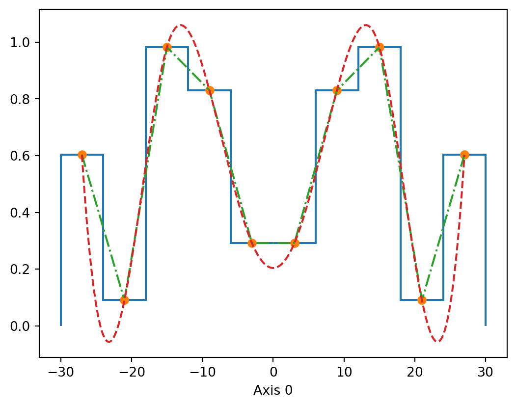
We can also plot them both together to compare the interpolations.
[7]:
h.plot()  # Plot the histogram
plt.plot(h.axes[0].centers, h.values(), "o")  # Mark the bin centers
plt.plot(x, linear_interp(x), "-.")  # Plot the Linear interpolation
plt.plot(x, cubic_interp(x), "--")  # Plot the Cubic interpolation
plt.show()