Hist Quick Demo#
My favorite demo notebook config setting:
[1]:
%config InteractiveShell.ast_node_interactivity="last_expr_or_assign"
Let’s import Hist:
[2]:
import numpy as np
from hist import Hist
We can use the classic constructors from boost-histogram, but let’s use the new QuickConstruct system instead:
[3]:
h = Hist.new.Reg(100, -10, 10, name="x").Double()
[3]:
Double() Σ=0.0
Let’s fill it with some data:
[4]:
h.fill(np.random.normal(1, 3, 1_000_000))
[4]:
Double() Σ=998519.0 (1000000.0 with flow)
And you can keep filling:
[5]:
h.fill(np.random.normal(-3, 1, 100_000))
[5]:
Double() Σ=1098519.0 (1100000.0 with flow)
You can plot (uses mplhep in the backend):
[6]:
h.plot();

We also have direct access to histoprint:
[7]:
h.show(columns=50)
-1.000 _ x 10^+01 26573/row ╷
-0.980 _
-0.960 _
-0.940 _
-0.920 _
-0.900 _
-0.880 _
-0.860 _
-0.840 _
-0.820 _
-0.800 _
-0.780 _
-0.760 _
-0.740 _
-0.720 _
-0.700 _█
-0.680 _█
-0.660 _█
-0.640 _█
-0.620 _██
-0.600 _██
-0.580 _███
-0.560 _███
-0.540 _████
-0.520 _█████
-0.500 _██████
-0.480 _███████
-0.460 _█████████
-0.440 _███████████
-0.420 _█████████████
-0.400 _████████████████
-0.380 _███████████████████
-0.360 _█████████████████████
-0.340 _████████████████████████
-0.320 _██████████████████████████
-0.300 _████████████████████████████
-0.280 _██████████████████████████████
-0.260 _██████████████████████████████
-0.240 _███████████████████████████████
-0.220 _████████████████████████████████
-0.200 _███████████████████████████████
-0.180 _████████████████████████████████
-0.160 _████████████████████████████████
-0.140 _█████████████████████████████████
-0.120 _█████████████████████████████████
-0.100 _█████████████████████████████████
-0.080 _███████████████████████████████████
-0.060 _████████████████████████████████████
-0.040 _█████████████████████████████████████
-0.020 _█████████████████████████████████████
0.000 _██████████████████████████████████████
0.020 _███████████████████████████████████████
0.040 _████████████████████████████████████████
0.060 _████████████████████████████████████████
0.080 _████████████████████████████████████████
0.100 _█████████████████████████████████████████
0.120 _████████████████████████████████████████
0.140 _████████████████████████████████████████
0.160 _████████████████████████████████████████
0.180 _████████████████████████████████████████
0.200 _███████████████████████████████████████
0.220 _██████████████████████████████████████
0.240 _████████████████████████████████████
0.260 _████████████████████████████████████
0.280 _██████████████████████████████████
0.300 _█████████████████████████████████
0.320 _████████████████████████████████
0.340 _██████████████████████████████
0.360 _█████████████████████████████
0.380 _███████████████████████████
0.400 _█████████████████████████
0.420 _███████████████████████
0.440 _██████████████████████
0.460 _████████████████████
0.480 _███████████████████
0.500 _█████████████████
0.520 _████████████████
0.540 _██████████████
0.560 _█████████████
0.580 _████████████
0.600 _██████████
0.620 _█████████
0.640 _████████
0.660 _███████
0.680 _██████
0.700 _██████
0.720 _█████
0.740 _████
0.760 _███
0.780 _███
0.800 _██
0.820 _██
0.840 _██
0.860 _█
0.880 _█
0.900 _█
0.920 _█
0.940 _
0.960 _
0.980 _
1.000 _
Let’s try 2D:
[8]:
h2 = Hist.new.Reg(100, -10, 10, name="x").Reg(100, -10, 10, name="y").Double()
[8]:
Regular(100, -10, 10, name='y')
Double() Σ=0.0
Can fill with two arrays:
[9]:
h2.fill(x=np.random.normal(-3, 2, 500_000), y=np.random.normal(3, 1, 500_000))
[9]:
Regular(100, -10, 10, name='y')
Double() Σ=499880.0 (500000.0 with flow)
Or a 2D array (hey, let’s do a multithreaded fill just for fun, too!):
[10]:
h2.fill(*np.random.normal(0, 5, (2, 10_000_000)), threads=4)
[10]:
Regular(100, -10, 10, name='y')
Double() Σ=9610472.0 (10500000.0 with flow)
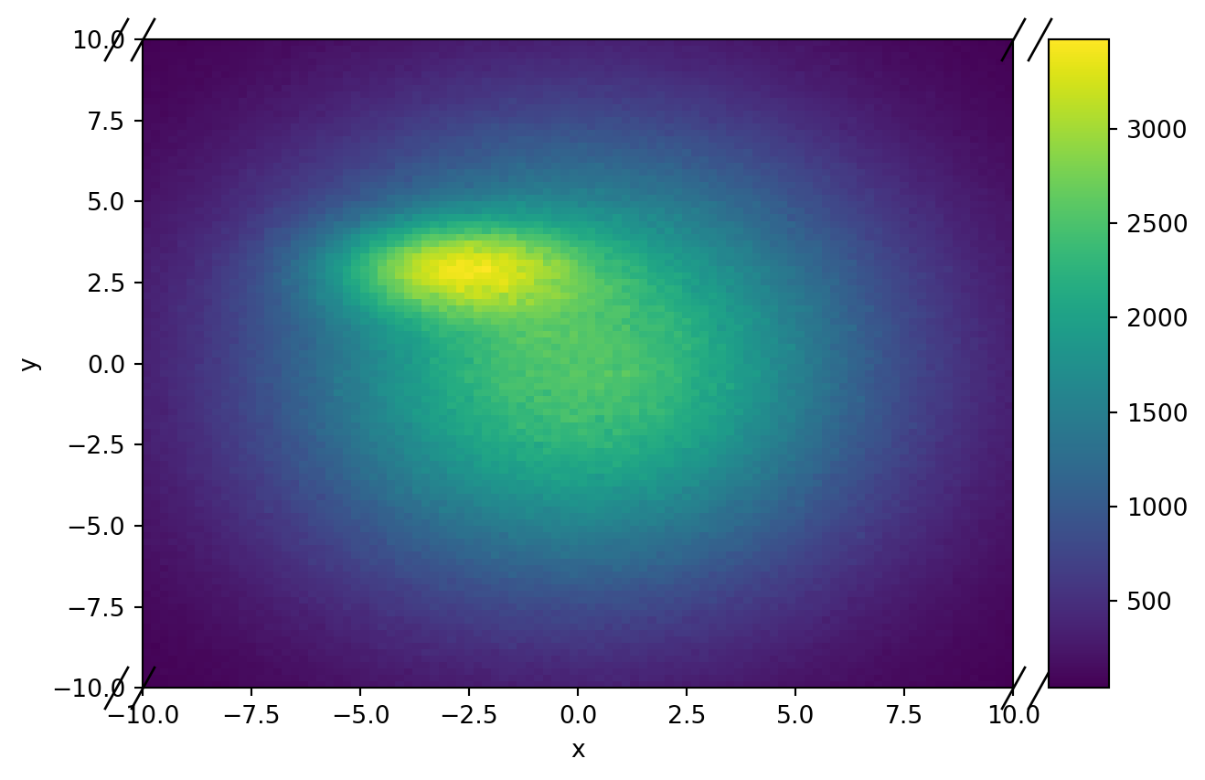
[11]:
h2.plot2d_full();
[12]:
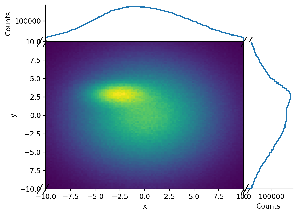
h2.plot();

[13]:
h2.project("x")
[13]:
Double() Σ=10044824.0 (10500000.0 with flow)
[14]:
h3 = (
Hist.new.Reg(100, -10, 10, name="x")
.Reg(50, -5, 5, name="y")
.Reg(60, -3, 3, name="z")
.Double()
)
[14]:
Hist(
Regular(100, -10, 10, name='x'),
Regular(50, -5, 5, name='y'),
Regular(60, -3, 3, name='z'),
storage=Double())
[15]:
h3.fill(*np.random.normal(0, 5, (3, 10_000_000)))
[15]:
Hist(
Regular(100, -10, 10, name='x'),
Regular(50, -5, 5, name='y'),
Regular(60, -3, 3, name='z'),
storage=Double()) # Sum: 2941613.0 (10000000.0 with flow)
[16]:
h3.project("x", "y")
# Can also write:
# h3[:, :, sum]
# h3[..., sum]
[16]:
Regular(50, -5, 5, name='y')
Double() Σ=6516265.0 (10000000.0 with flow)
We can slice and dice. Plain numbers refer to bins. Use a “j” suffix to refer to data coordinates. As above, sum will sum over an axis (optionally with end points). This system is called UHI+.
[17]:
h3[-8j:8j, 10:50, sum]
[17]:
Regular(40, -3, 5, name='y')
Double() Σ=5050592.0 (10000000.0 with flow)
You can also use a dict; that includes using names too. (Note: this was independently developed but is nearly identical to XArray)
[18]:
h3[{"x": slice(-8j, 8j), "y": slice(10, 50), "z": sum}]
[18]:
Regular(40, -3, 5, name='y')
Double() Σ=5050592.0 (10000000.0 with flow)
Everything integrates with histoprint, uproot4, and mplhep, too:
[19]:
import mplhep
[20]:
mplhep.hist2dplot(h2);